PE Study
Initial Processing
Change types and rename
df_model <- df_model %>% rename(Severity = PE.Severity.1.low.risk..2.intermediate..3.massive..4.indeterminate)
df_model$type <- as.factor(df_model$type)
df_model$Gender <- as.factor(df_model$Gender)
df_model$Race <-as.factor(df_model$Race)
df_model$BOVA.Score <- as.factor(df_model$BOVA.Score)
Filter for low risk patients by PE Severity
df_all <- df_model %>% filter(Severity < 3)
df_all$Severity <- as.factor(df_all$Severity)
Bin by age
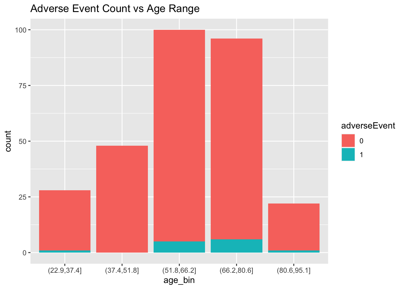
breaks = 5
df_all$age_bin <- cut(df_all$Age, breaks=breaks)
What constitutes an Adverse Event?
- Death, either in hospital or within 30 days of release
- Arrhythmia that required treatment
- Inotropes
- Vasopressors
- Use of Non-Rebreather mask
- Shock
- ACLS
- Intubation
- tPA
- Transfusion
- EKOS
Visualize Distributions
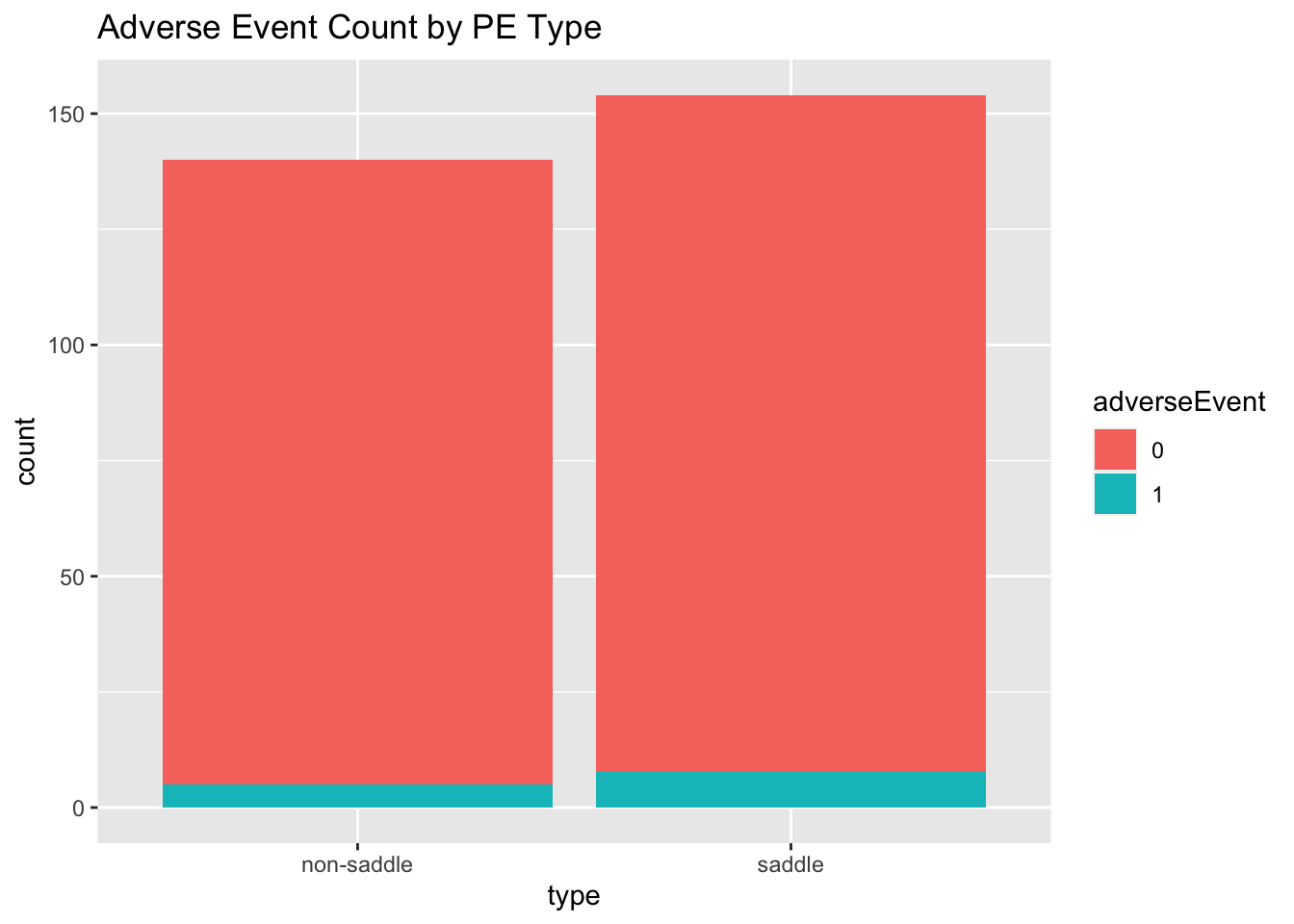
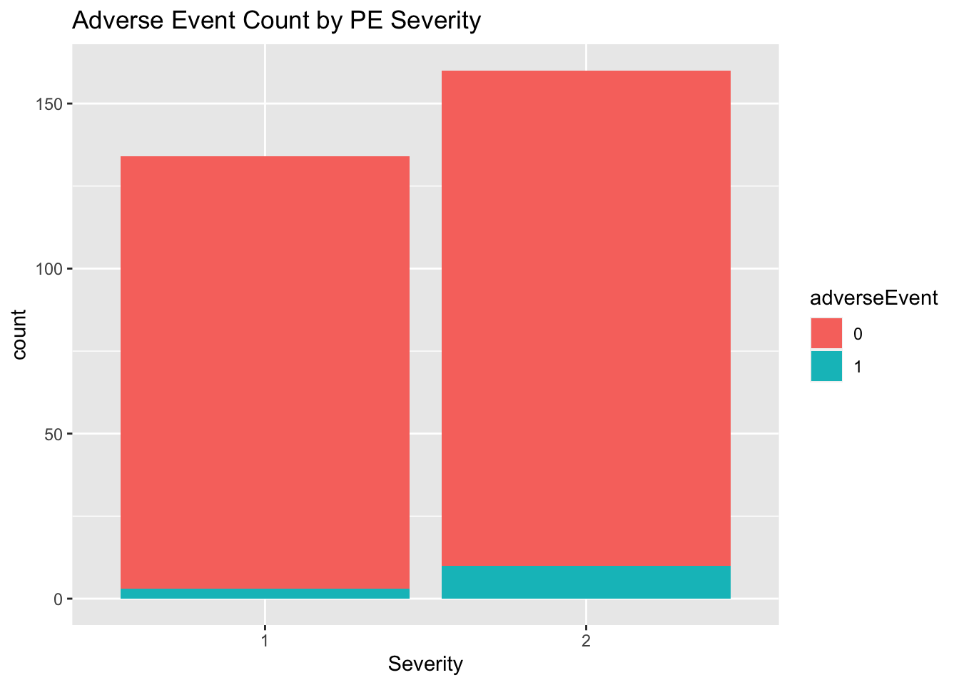
Severity is a potential confounder, noticing the slight correlation with adverse event rates
2x2 Tables
2x2 Table for entire cohort
# table_group <- table(df_all$adverseEvent, df_all$type, df_all$age_bin)
test_mat <- as.matrix(table(df_all$type, df_all$adverseEvent))
test_mat
##
## 0 1
## non-saddle 135 5
## saddle 146 82x2 Table for cohort, by PE Severity
table(df_all$type, df_all$adverseEvent, df_all$Severity)## , , = 1
##
##
## 0 1
## non-saddle 94 1
## saddle 37 2
##
## , , = 2
##
##
## 0 1
## non-saddle 41 4
## saddle 109 6Check for confounding
m_crude <- glm(formula = 'adverseEvent ~ type', data = df_all, family = binomial)
summary(m_crude)
##
## Call:
## glm(formula = "adverseEvent ~ type", family = binomial, data = df_all)
##
## Deviance Residuals:
## Min 1Q Median 3Q Max
## -0.3266 -0.3266 -0.2697 -0.2697 2.5816
##
## Coefficients:
## Estimate Std. Error z value Pr(>|z|)
## (Intercept) -3.2958 0.4554 -7.237 4.59e-13 ***
## typesaddle 0.3917 0.5825 0.672 0.501
## ---
## Signif. codes: 0 '***' 0.001 '**' 0.01 '*' 0.05 '.' 0.1 ' ' 1
##
## (Dispersion parameter for binomial family taken to be 1)
##
## Null deviance: 106.50 on 293 degrees of freedom
## Residual deviance: 106.04 on 292 degrees of freedom
## AIC: 110.04
##
## Number of Fisher Scoring iterations: 6m_adj <- glm(formula = 'adverseEvent ~ type + Age + Severity + Race + Gender', data = df_all, family = binomial)
summary(m_adj)##
## Call:
## glm(formula = "adverseEvent ~ type + Age + Severity + Race + Gender",
## family = binomial, data = df_all)
##
## Deviance Residuals:
## Min 1Q Median 3Q Max
## -0.5006 -0.3600 -0.2568 -0.1984 2.7476
##
## Coefficients:
## Estimate Std. Error z value Pr(>|z|)
## (Intercept) -19.05928 3956.18053 -0.005 0.996
## typesaddle 0.08057 0.62988 0.128 0.898
## Age 0.02755 0.02139 1.288 0.198
## Severity2 0.94037 0.72126 1.304 0.192
## RaceB 13.57175 3956.18041 0.003 0.997
## RaceH -1.23444 4805.32103 0.000 1.000
## RaceNH -1.14524 4322.76564 0.000 1.000
## Racerefused -0.65935 5594.88396 0.000 1.000
## RaceW 13.50987 3956.18040 0.003 0.997
## GenderM 0.11571 0.60291 0.192 0.848
## GenderM -14.69737 3956.18039 -0.004 0.997
##
## (Dispersion parameter for binomial family taken to be 1)
##
## Null deviance: 106.50 on 293 degrees of freedom
## Residual deviance: 100.55 on 283 degrees of freedom
## AIC: 122.55
##
## Number of Fisher Scoring iterations: 16Calculate percent change in typesaddle coefficient between models. If absolute value is greater than 10%, confounding needs to be adjusted for.
beta_crude <- coefficients(m_crude)[['typesaddle']]
beta_adj <- coefficients(m_adj)[['typesaddle']]
(beta_adj - beta_crude) / beta_crude
## [1] -0.794297Confounding is present, however the GLM models suggest that there is no relationship between adverse event rates and PE type (saddle vs non-saddle)
Compare to VGAM package outputs for sanity check
m_vgam <- vglm(formula = 'adverseEvent ~ type + Age + Severity + Race + Gender', binomialff(link = "logitlink"), data = df_all)
coefficients(m_vgam)[['typesaddle']]
## [1] 0.08056805The predictor “type” is confounded by adding in further predictors such as Age, Severity, and Race. Severity alone is the most powerful confounder and should be controlled for. We will use the Cochran-Mantel-Haenszel to account for the observed confounding effect of Severity.
Hypothesis test is set based on what constitutes surprise for the doctor.
H0: There is no difference in the adverse event odds ratio of saddle vs non-saddle in severity controlled groups
H1: There is a difference in the adverse event odds ratio of saddle vs non-saddle in severity controlled groups
Odds ratio in this case is defined as…
(saddle adverse event count / saddle no adverse event count) / (non-saddle adverse event count / non-saddle no adverse event count)
Test 1: Fisher’s exact test for entire cohort
m_fisher <- exact2x2(test_mat, conf.level = 0.99)
m_fisher
##
## Two-sided Fisher's Exact Test (usual method using minimum likelihood)
##
## data: test_mat
## p-value = 0.5782
## alternative hypothesis: true odds ratio is not equal to 1
## 99 percent confidence interval:
## 0.3357 7.6156
## sample estimates:
## odds ratio
## 1.477511Based on test results, we do not reject the null hypothesis, however we will still control for confounding factor of PE Severity. Use the Cochran-Mantel-Haenszel test.
Test 2: Cochran-Mantel-Haenszel test to control for PE Severity
m_cmh <- mantelhaen.test(table(df_all$type, df_all$adverseEvent, df_all$Severity), exact = TRUE)
m_cmh
##
## Exact conditional test of independence in 2 x 2 x k tables
##
## data: table(df_all$type, df_all$adverseEvent, df_all$Severity)
## S = 135, p-value = 1
## alternative hypothesis: true common odds ratio is not equal to 1
## 95 percent confidence interval:
## 0.2456193 4.3600803
## sample estimates:
## common odds ratio
## 0.976237We notice that after controlling for PE Severity in submassive patients, there is no evidence to suggest a statistically significant or practically significant difference in the adverse event counts between saddle and non-saddle pulmonary embollism.
Control for multiple comparisons using Benjamini & Yekutieli correction
pvalues <- c(m_fisher$p.value, m_cmh$p.value)
p.adjust(pvalues, method = "BY")
## [1] 1 1Given the multiple comparisons correction, and our alpha value of 1%, both tests have given p-values where we cannot reject the null hypothesis in favor of the alternate hypothesis. The common odds ratio confidence interval for adverse events in saddle over non-saddle is…
0.2456193, 4.3600803
Submassive Patients with Saddle PE are no more likely to experience an adverse event as those with Non-Saddle PE
How predictive are PESI, sPESI, and BOVA?
m_pred_spesi <- glm(formula = 'adverseEvent ~ sPESI', data = df_model, family = binomial)
PseudoR2(m_pred_spesi, which = 'McKelveyZavoina')
## McKelveyZavoina
## 0.3473808summary(m_pred_spesi)##
## Call:
## glm(formula = "adverseEvent ~ sPESI", family = binomial, data = df_model)
##
## Deviance Residuals:
## Min 1Q Median 3Q Max
## -0.5105 -0.5105 -0.5105 -0.1310 3.0861
##
## Coefficients:
## Estimate Std. Error z value Pr(>|z|)
## (Intercept) -4.754 1.004 -4.733 2.21e-06 ***
## sPESI 2.782 1.025 2.714 0.00666 **
## ---
## Signif. codes: 0 '***' 0.001 '**' 0.01 '*' 0.05 '.' 0.1 ' ' 1
##
## (Dispersion parameter for binomial family taken to be 1)
##
## Null deviance: 193.1 on 337 degrees of freedom
## Residual deviance: 175.6 on 336 degrees of freedom
## AIC: 179.6
##
## Number of Fisher Scoring iterations: 7m_pred_pesi <- glm(formula = 'adverseEvent ~ PESI.Class', data = df_model, family = binomial)
PseudoR2(m_pred_pesi, which = 'McKelveyZavoina')## McKelveyZavoina
## 0.3012967summary(m_pred_pesi)##
## Call:
## glm(formula = "adverseEvent ~ PESI.Class", family = binomial,
## data = df_model)
##
## Deviance Residuals:
## Min 1Q Median 3Q Max
## -0.7894 -0.3462 -0.2239 -0.1441 3.0242
##
## Coefficients:
## Estimate Std. Error z value Pr(>|z|)
## (Intercept) -5.4515 0.7631 -7.144 9.04e-13 ***
## PESI.Class 0.8890 0.1842 4.826 1.39e-06 ***
## ---
## Signif. codes: 0 '***' 0.001 '**' 0.01 '*' 0.05 '.' 0.1 ' ' 1
##
## (Dispersion parameter for binomial family taken to be 1)
##
## Null deviance: 193.10 on 337 degrees of freedom
## Residual deviance: 162.67 on 336 degrees of freedom
## AIC: 166.67
##
## Number of Fisher Scoring iterations: 6m_pred_bova <- glm(formula = 'adverseEvent ~ BOVA.Score', data = df_model, family = binomial)
PseudoR2(m_pred_bova, which = 'McKelveyZavoina')## McKelveyZavoina
## 0.9658163summary(m_pred_bova)##
## Call:
## glm(formula = "adverseEvent ~ BOVA.Score", family = binomial,
## data = df_model)
##
## Deviance Residuals:
## Min 1Q Median 3Q Max
## -0.60386 -0.34305 -0.31495 -0.00005 2.62068
##
## Coefficients:
## Estimate Std. Error z value Pr(>|z|)
## (Intercept) -2.8034 0.7282 -3.850 0.000118 ***
## BOVA.Score0 -17.7627 1722.1259 -0.010 0.991770
## BOVA.Score1 1.0116 0.9587 1.055 0.291366
## BOVA.Score2 -0.1756 0.9384 -0.187 0.851590
## BOVA.Score3 0.2384 1.0338 0.231 0.817615
## BOVA.Score4 -0.5978 1.2505 -0.478 0.632582
## BOVA.Score5 1.0986 0.8528 1.288 0.197663
## BOVA.Score7 1.1939 1.3154 0.908 0.364067
## BOVA.Scoredoes not qualify for scoring, SBP <90 23.3694 12537.2648 0.002 0.998513
## BOVA.Scoredoes not quality for scoring, BP <90 23.3694 6701.4500 0.003 0.997218
## BOVA.Scoredoes not quality for scoring, SBP <90 23.3694 17730.3699 0.001 0.998948
## ---
## Signif. codes: 0 '***' 0.001 '**' 0.01 '*' 0.05 '.' 0.1 ' ' 1
##
## (Dispersion parameter for binomial family taken to be 1)
##
## Null deviance: 193.10 on 337 degrees of freedom
## Residual deviance: 118.72 on 327 degrees of freedom
## AIC: 140.72
##
## Number of Fisher Scoring iterations: 19Both sPESI and PESI Class are significant predictors of adverse event rates and have similar predictive power. Surprisingly, BOVA score has a high Pseudo R2 value, as well as having a lower AIC value compared to sPESI and PESI, suggesting that it is a better diagnostic tool for predicting adverse events than sPESI or PESI are.